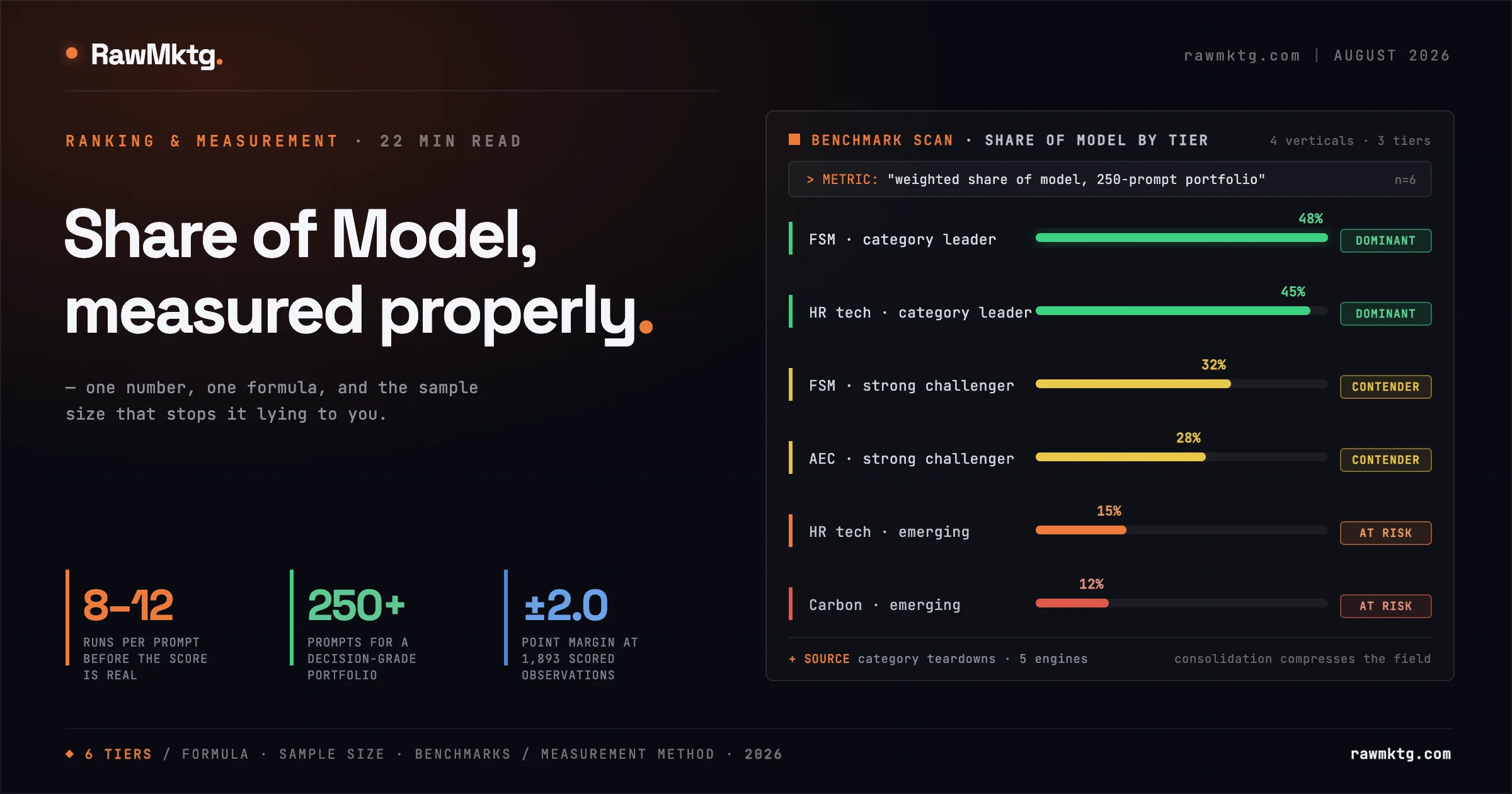
Most teams find out about their AI visibility the same way. Someone on the exec team types the category question into ChatGPT, does not see the company, and forwards the screenshot to marketing. That screenshot is not data. It is one draw from a probability distribution, and the next person to type the same question will get a different answer.
This article is the worked spec. The one-page, versioned standard every rawmktg figure follows lives at the measurement methodology.
Share of Model is the metric that replaces the screenshot. It answers one question with one number: across the questions your buyers actually ask, in the engines they actually use, how much of the answer space do you own compared to everyone else selling into the same problem. This piece is the methodology, not the taxonomy and not the attribution plumbing, just the metric, how to compute it, how big a sample it needs, and how to read the result. A single number can still hide which buying stage is missing, which is why a segment teardown reports four measures, not one.
Share of Model = your weighted presence divided by the total weighted presence of every brand in the category, computed over the same prompt portfolio, on the same engines, on a fixed cadence.
What makes it hard is not the mathematics, it is the discipline: a fixed portfolio, enough runs, honest weights, and the willingness to publish a number lower than the one your tool vendor reports.
01How do the three AI-visibility metrics differ?
Before you can count anything, you have to decide what counts. A brand name in a paragraph, a URL in a footnote, and a brand named as the recommendation are three different events with three different causes, the distinction drawn in citation vs mention vs recommendation, and it is upstream of everything here. Once you know a brand appeared, you still need to know whether that answer produced a session or a deal, a plumbing problem covered in prompt-to-citation tracking. Share of Model sits between them: it is a scoreboard, not a diagnosis and not a revenue model.
| Metric | What it counts | Unit | Fails when |
|---|---|---|---|
| Share of Voice | Media impressions and paid reach | Impressions | Buyers stop seeing media and start asking a model |
| Share of Search | Branded query volume in Google | Search volume | The query never reaches Google because the answer arrived first |
| Rank tracking | Position on a static results page | Position 1 to 100 | There is no page, only a synthesized paragraph |
| Share of Model | Weighted brand presence in generated answers | Percent of answer space | The prompt set is too small or unweighted |
The last row is the whole argument. Generative outputs are probabilistic, so the correct unit of measurement is a share of a distribution, not a position on a list.
02What does Share of Model actually measure?
A statistically representative set is a fixed portfolio, versioned and re-run identically each cycle, covering the range of ways a buyer actually phrases the problem. If the portfolio changes between cycles, the trend line is meaningless. Across multiple engines matters because ChatGPT, Perplexity, Google AI Overviews, Claude and Grok retrieve, and therefore recommend, differently, the reason set out in why different engines recommend different vendors; a blended single number hides the fact that you might own one engine and be invisible in another.
Weighted by intent is the part most tools skip. A brand named in answer to "what is workforce management software" and a brand named in answer to "which workforce management platform handles multi-state overtime compliance under $12 per employee" are not worth the same. One is a definition. The other is a shortlist that ends in a purchase order.
03Why does the naive inclusion-rate formula lie to you?
Nearly every tool that reports an AI-visibility score starts with the unweighted inclusion rate: the number of responses in which the brand appears anywhere, divided by the total scored responses. Show up in 620 of 2,000 answers and you score 31%. It treats a fourth-alternative caveat mention identically to being named the single best option; it treats a Grok mention the same as an enterprise-procurement ChatGPT mention; and it rewards you for winning cheap definitional prompts that are worth almost nothing.
Brand A is winning the definitional long tail and appearing late in lists. Brand B appears less often but appears first, in comparison and constraint prompts, in the engines its buyers use. A raw count says Brand A leads by seven points; the weighted score says Brand B leads by nineteen. Only one of those conclusions would survive contact with the pipeline, which is the same gap between ranking and visibility.
04What is the formula that holds up?
SoM(b) =    Σ_e  Σ_p   w_e · w_p · score(b, e, p)
           -----------------------------------------
           Σ_{b' in C}  Σ_e  Σ_p   w_e · w_p · score(b', e, p)

  w_e     engine weight, Σ w_e = 1   (where your buyers ask)
  w_p     intent weight, 0.5x .. 2.0x (distance from purchase)
  score   presence in [0,1], averaged over N runs of the prompt
  C       the competitive set (the denominator is field presence,
          not response count, that is what makes it a share)
Setting the engine weights
Engine weight is a business decision, not a statistical one: it reflects where your buyers ask, not global market share. A B2B infrastructure vendor selling to platform engineers weights Perplexity and Claude higher; a mid-market SaaS company selling to operations leaders weights ChatGPT and Google AI Overviews heavily. Set the weights once, document the reasoning, and do not change them mid-year. If you must revise them, restate prior periods on the new weights so the trend stays honest.
Setting the intent weights
Intent weight scales with distance from a purchase decision. A workable default we use across teardowns:
| Intent tier | Weight | What the prompt is doing | Example |
|---|---|---|---|
| Navigational & entity | 0.5x | Testing whether the model knows you exist and describes you correctly | What is Acme, and what does it do? |
| Category discovery | 1.0x | Unbranded category ask, no vendor named | Best workforce management platforms for multi-site healthcare |
| Comparative & evaluation | 1.5x | Head-to-head, pros and cons, shortlist construction | Compare Acme and Beta for compliance tracking |
| Transactional & constraint | 2.0x | Hard budget, integration or regulatory constraints attached | HRIS under $15 per employee with Slack and SOC 2 Type II |
The gap between 0.5 and 2.0 is deliberate. It is the difference between a model knowing your name and a model putting you on a shortlist while the buyer has a budget open. Brands that only optimize the top of that table build an authority position with no demand attached.
05How do you score a single response?
| Dimension | Symbol | Weight | What it captures |
|---|---|---|---|
| Mention inclusion | m | 0.30 | Is the brand named or cited anywhere in the response. Binary. |
| Recommendation endorsement | d | 0.30 | Presented as a pick rather than a passing reference. Active endorsements carry 3-5x the value of a co-mention. |
| Position prominence | rho | 0.20 | Where in the answer hierarchy the brand lands. Graded, not binary. |
| Sentiment polarity | s | 0.15 | Positive framing scores 1.0, neutral 0.6, negative 0.0. |
| Entity accuracy | a | 0.05 | Are the stated features, pricing and positioning correct. Catches hallucination. |
Position prominence needs a ladder rather than a raw rank, because the drop-off is not linear, being named first is worth far more than twice being named second. Entity accuracy carries the smallest weight but the largest downside: a brand can score well on inclusion and still be harmed if the model consistently misstates its pricing tier, so track it as a separate alarm, not just a 5% input. The structural fix is in hallucination-proofing your brand.
from dataclasses import dataclass

POSITION_WEIGHTS = {1: 1.00, 2: 0.70, 3: 0.70, 4: 0.40, 5: 0.40, 6: 0.40}
TAIL_WEIGHT      = 0.15
SENTIMENT        = {"positive": 1.0, "neutral": 0.6, "negative": 0.0}
DIM_WEIGHTS      = {"m": 0.30, "d": 0.30, "rho": 0.20, "s": 0.15, "a": 0.05}

@dataclass
class Extraction:
    rank: int; mentioned: int; recommended: int
    sentiment: str; entity_accurate: int

def presence(x):
    rho = POSITION_WEIGHTS.get(x.rank, TAIL_WEIGHT)
    return (DIM_WEIGHTS["m"]   * x.mentioned
          + DIM_WEIGHTS["d"]   * x.recommended
          + DIM_WEIGHTS["rho"] * rho
          + DIM_WEIGHTS["s"]   * SENTIMENT[x.sentiment]
          + DIM_WEIGHTS["a"]   * x.entity_accurate)

# average presence() over the N runs of the prompt. keep the weights
# in config, not in code, so a weighting change is auditable.
Extraction is the part people underestimate. Brand names get truncated, pluralized and abbreviated inside generated prose. Build an alias table per brand before you run anything, and validate your extractor against a hand-labelled sample of at least 200 responses before you trust a single score.
06How many runs per prompt do you actually need?
At one run your estimate is either 0% or 100%. At three runs it can still be off by 30 points. Somewhere around eight to twelve runs per prompt per engine, the estimate settles into a range you can act on. Perplexity and Google AI Overviews are especially unstable because they re-retrieve on every call.
Bounding the estimate
Report intervals, not point estimates. For simple presence proportions use a Wilson score interval rather than the normal approximation, which breaks badly at the low rates most brands actually have.
import math

def wilson(successes, n, z=1.96):
    """95% CI for a proportion. Correct at small n and extreme p,
    where the normal approximation breaks badly."""
    if n == 0:
        return (0.0, 0.0)
    p      = successes / n
    denom  = 1 + z*z / n
    centre = (p + z*z / (2*n)) / denom
    margin = z * math.sqrt(p*(1-p)/n + z*z/(4*n*n)) / denom
    return (centre - margin, centre + margin)   # use for inclusion rates
The weighted Share of Model composite is not a simple proportion, and mentions cluster inside multi-brand responses, which violates the independence Wilson assumes. For the composite, resample at the response level with a percentile bootstrap.
import numpy as np

def bootstrap_som(responses, brand, n_iter=1000, seed=7):
    """Percentile bootstrap CI for the weighted composite. Resample
    whole responses, not individual mentions, so within-response
    correlation (brands cluster inside multi-brand answers) survives."""
    rng = np.random.default_rng(seed)
    idx = np.arange(len(responses))
    est = []
    for _ in range(n_iter):
        sample = [responses[i] for i in rng.choice(idx, len(idx))]
        est.append(weighted_som(sample, brand, ENGINE_W, INTENT_W))
return tuple(np.percentile(est, [2.5, 97.5])) # <1000 iters = unstable tails07How many prompts do you need?
n = z² · p(1 - p) / E²

  z = 1.96  (95% confidence)
  p = 0.27  (observed inclusion rate)
  E = 0.02  (target margin of error, ±2 points)

  ->  n ≈ 1,896 scored observations, per brand, per engine
  at 10 runs/prompt that is ≈ 190 prompts; round up to a
  250 to 500 prompt portfolio, run 5 to 12 times per engine.
The flattening matters more than the absolute numbers. Going from 500 to 2,500 observations buys a large precision gain; going from 2,500 to 5,000 buys very little. That is the argument for a 250-prompt portfolio rather than a 500-prompt one if budget is tight, spend the saved API calls on more engines instead.
A 50 to 100 prompt audit is fine for a first look and for finding obvious gaps. It is not enough to declare a winner between two brands sitting three points apart, and it is not enough to claim a quarter-over-quarter improvement. Say which one you are doing.
08Why can't you blend the engines into one number?
| Engine | Primary retrieval | Variance | Min runs | Best intent fit |
|---|---|---|---|---|
| ChatGPT | Hybrid parametric plus web RAG | Moderate | 10 | Broad commercial and B2B discovery |
| Perplexity | Live web RAG indexing | High | 12 | Deep technical and research queries |
| Google AI Overviews | Search graph plus Gemini | High | 10 | High-volume consumer and business search |
| Claude | Parametric-heavy, extended context | Low to moderate | 8 | Long-form analysis and enterprise evaluation |
| Grok | Real-time social plus web RAG | High | 12 | Real-time trends and industry news |
A brand strong on Claude and weak on Perplexity has a live-retrieval problem: the training corpus knows it, the live index does not. That is a crawlability and freshness fix, not a brand fix, and the mechanics are in how your page gets retrieved.
09How do you build the prompt portfolio?
Most buyer phrasings have zero search volume, which is exactly why the query fan-out mechanics matter here. A workable split is 15% navigational, 35% category discovery, 30% comparative and 20% transactional. Discovery gets the largest share because it is where the category conversation happens; transactional gets the highest weight because it is where the money is.
# portfolio.yaml -- version this file. It IS the measurement instrument.
version: 2026.Q3.1
category: field_service_management
competitor_set: [acme, beta, gamma, delta, epsilon, zeta]

engine_weights:              # must sum to 1.0 -- where your buyers ask
  chatgpt:      0.38
  ai_overviews: 0.24
  perplexity:   0.18
  claude:       0.12
  grok:         0.08

intent_weights: {navigational: 0.5, discovery: 1.0,
                 comparative: 1.5, transactional: 2.0}

prompts:
  - {id: fsm-disc-001, tier: discovery,     text: "best field service software for HVAC"}
  - {id: fsm-comp-014, tier: comparative,   text: "ServiceTitan vs Housecall Pro for a 40-tech shop"}
  - {id: fsm-txn-031,  tier: transactional, text: "FSM under $80/tech/mo with QuickBooks + SOC 2"}
Three rules keep the instrument honest. Never edit a prompt in place, deprecate it and add a new ID. Never add prompts mid-cycle, batch them into the next version. Always keep at least 80% of prompts stable across versions so the trend line survives.
10What does the measurement pipeline look like?
from collections import defaultdict

def weighted_som(responses, brand, engine_w, intent_w):
    """responses: iterable of scored responses across the portfolio."""
    num = den = 0.0
    for r in responses:
        w    = engine_w[r.engine] * intent_w[r.tier]
        num += w * r.scores.get(brand, 0.0)
        den += w * sum(r.scores.values())   # total field presence
    return num / den if den else 0.0        # a share, not a rate
Storage is cheaper than execution by two orders of magnitude, so keep the full text of every response, not the extraction. And the rollup query's guard clause is not optional: under-sampled cells are the main source of fake movement.
-- Cycle-over-cycle movement, ready for the dashboard.
WITH scored AS (
  SELECT cycle_id, engine, tier, brand,
         engine_weight * intent_weight * presence_score AS w_score,
         engine_weight * intent_weight * field_score    AS w_field
  FROM   response_scores
  WHERE  portfolio_version = '2026.Q3.1'
)
SELECT cycle_id,
       SUM(w_score) / NULLIF(SUM(w_field), 0) AS share_of_model,
       COUNT(*)                               AS observations
FROM   scored
GROUP  BY cycle_id
HAVING COUNT(*) >= 200;   -- the HAVING is not optional: under-sampled
-- cells are the main source of fake movement.11What does a good Share of Model score look like?
| Vertical | Category leader | Strong challenger | Emerging provider | What drives retrieval |
|---|---|---|---|---|
| HR tech & staffing | 35-45% | 18-30% | 5-15% | Directory reviews (G2, Capterra), community forums, pricing pages |
| AEC services & tech | 32-42% | 15-28% | 4-12% | Technical specs, trade association journals, Schema.org entities |
| Field service management | 38-48% | 20-32% | 5-14% | Feature comparison tables, integration guides, industry reviews |
| Carbon accounting | 35-45% | 16-28% | 3-12% | Methodological papers, GHG Protocol citations, regulatory briefs |
Three things to read out of that table. Field service runs highest at the top because it is the most consolidated, so the leader's denominator is smaller, the full breakdown is in the field service software teardown. Carbon accounting runs lowest because the category rewards methodological credibility over marketing volume, which a new entrant cannot buy quickly, we took that market apart in authority isn't the moat. And the retrieval-driver column is the actionable one: optimizing an AEC site with HR-tech tactics produces nothing.
The tier that surprises people is the bottom one. In our lending and credit teardown, 44 of 52 brands were named 0% of the time. Not low, zero, a large fraction of a well-funded category sitting entirely outside the answer space. Movement is slower than teams expect: set expectations at three to five points per quarter for a brand in the emerging tier doing the work consistently.
12How do you connect model share to money?
The authority-gap map, the third-party domains engines cite for your category where you are absent, is your outreach target list, and the method is in authority seeding for AI. Two formulas carry the budget conversation. Return on GEO connects spend to tracked revenue plus a conservatively attributed brand-lift term, and cost of inaction quantifies the gap to the leader as forgone pipeline.
A field service platform running at 14% against a leader at 38%, in a category generating an estimated 120,000 relevant prompts a year, converting AI-sourced exposure at 1.4% into opportunities worth an average of $18,000. The 24-point gap maps to 28,800 answers, which maps to roughly $7.26 million in annual pipeline that goes to someone else.
Be honest about what that number is: a sizing estimate built on a conversion assumption you should state explicitly, not a forecast. Its job is to make the gap legible to a CFO, not to be booked.
13How do you stand the program up in 90 days?
| Stage | Focus | Deliverables |
|---|---|---|
| Days 1-14 | Baseline audit | Curate the 250+ prompt portfolio, run first sampling across five engines, map competitor Share of Model |
| Days 15-30 | Machine scannability | llms.txt at root, clean Markdown variants, Schema.org markup, verify bot access in robots.txt |
| Days 31-60 | Citation-gap acquisition | Targeted PR and placement on the high-citation third-party domains from authority mapping |
| Days 61-75 | Pipeline attribution | GA4 referral tracking for AI engines, dashboard combining Share of Model and referral conversions |
| Days 76-90 | Operational cadence | Automated monthly polling, variance alerts, Share of Model in the quarterly review |
Days 15 to 30 come before the authority work for a reason: if the crawlers cannot parse your pages, the placements you earn in days 31 to 60 will feed engines that still cannot retrieve your site, and you will pay for coverage that only helps your competitors' answers look better sourced. Check crawler behaviour first, using the breakdown in how AI crawlers actually index your site.
14What are the seven ways the number goes wrong?
| Failure | What it looks like | Fix |
|---|---|---|
| Single-run sampling | Score swings 15 points between cycles with no work done | 8 to 12 runs per prompt per engine, minimum |
| Portfolio drift | Prompts edited or added between cycles | Version the portfolio file, keep 80% stable, deprecate rather than edit |
| Blended-only reporting | One number that hides an engine you are invisible in | Always publish the per-engine cut alongside the headline |
| Alias misses | Extractor misses abbreviations and truncations of the brand | Alias table per brand, validated against 200 hand-labelled responses |
| Weight tinkering | Score improves after a weighting change, not after work | Freeze weights for the year, restate history if you must revise |
| Under-sampled cells | A tier or engine with 40 observations reported as a trend | Suppress cells below a minimum observation count |
| Denominator confusion | Reporting a rate and calling it a share | Denominator is total field presence across the competitor set, not response count |
If your weights change, the previous quarter has to be restated on the new weights before anyone sees a trend line. Write that into the process document.
15What should you do this week?
- Settle the taxonomy first. Decide what counts as a citation, a mention and a recommendation before you count anything, using the taxonomy piece as the reference.
- Write 50 prompts from sales-call notes, not from a keyword tool, and tag each to an intent tier. This is your pilot portfolio.
- Run each prompt 10 times on two engines. Score presence with the five dimensions and report the number with a Wilson interval attached.
- Compare to the band for your vertical and tier in Table 5. If you are below the emerging band, the problem is retrieval, not messaging.
- Pull the citation-source split. If more than 70% of your citations come from your own domain, the authority gap is your first project.
- Freeze the weights, version the portfolio, and put the next run on the calendar. A single measurement is a screenshot; two comparable measurements are a program.
Share of Model is not complicated mathematics. It is a weighted average with confidence intervals attached. What makes it hard is the discipline, a fixed portfolio, enough runs, honest weights, and the willingness to publish a number lower than the one your tool vendor reports. That discipline is the entire difference between measurement and guessing.
Frequently asked questions
What is Share of Model tracking, and do you need an agency for it?
Share of Model tracking is measuring, on a fixed cadence, how often and how prominently a brand is named across AI answers for a category, then trending it over time. You do not need a Share of Model agency to start: the method is a frozen prompt portfolio run 8 to 12 times per engine with the results scored and bounded, which an in-house team can run themselves. An agency mainly helps with scale and consistency, not with anything proprietary; the full standard is public on the measurement methodology page.
What is Share of Model and how is it calculated?
Share of Model is the percentage of brand presence an entity captures across a statistically representative set of category prompts, measured across multiple generative engines and weighted by commercial intent and engine usage. You compute it as your weighted presence divided by the total weighted presence of every brand in the competitive set, over the same prompt portfolio, on the same engines, on a fixed cadence. The denominator is total field presence, not response count, which is what makes it a share rather than a rate.
How many times should you run each prompt?
Eight to twelve runs per prompt per engine, minimum. Language models are probabilistic: the same prompt sent twice can return different brand sets. At one run your estimate is either 0% or 100%; at three runs it can still be off by 30 points; the estimate only settles into an actionable range around eight to twelve runs. High live-retrieval engines like Perplexity and Google AI Overviews need the top of that range because they re-retrieve on every call.
How many prompts do you need for a reliable Share of Model?
To hold a two-point margin of error at a 27% inclusion rate you need roughly 1,900 scored observations per brand per engine. At ten runs per prompt that is about 190 prompts, so decision-grade programmes land at a portfolio of 250 to 500 prompts run 5 to 12 times per engine. Precision flattens hard after about 2,500 observations, so a 250-prompt portfolio plus more engines usually beats a 500-prompt one on a tight budget.
Should you report one blended AI-visibility number across engines?
Report both, but never blended-only. The weighted composite goes on the dashboard; the per-engine breakdown goes in the appendix, because that is where the fix lives. A brand strong on Claude and weak on Perplexity has a live-retrieval problem, the training corpus knows it but the live index does not, which is a crawlability and freshness fix rather than a brand fix. A single blended number hides the engine you are invisible in.
What is a good Share of Model score?
It depends entirely on the vertical and your competitive tier, so a raw number means nothing in isolation. Across teardowns brands land in four tiers: category leaders run roughly 35-48%, strong challengers 15-32%, and emerging providers 3-15%, with the exact bands set by how consolidated the market is. Field service tops out highest (leader band to 48%) because it is the most consolidated; carbon accounting bottoms lowest (emerging to 3%) because engines there reward peer-reviewed and regulatory sources over marketing volume. Read your number against the band for your tier.
How is Share of Model different from share of voice, citations and mentions?
Share of voice counts media impressions; share of search counts branded query volume; both break when the buyer asks a model instead of seeing an ad or reaching Google. Citations, mentions and recommendations are the underlying events, a taxonomy that is upstream of Share of Model and defines what you count. Share of Model is the middle scoreboard layer: it takes those events, counts them across a fixed weighted prompt portfolio, and turns them into one share you can trend and benchmark. Attribution to sessions and pipeline is a separate downstream layer.
Figures 1 through 14 are original, built from the data and formulas in the sources below.
- Share of Model, Generative Engine Optimization. Alephic.
- Share of Model Framework: Architectonics of Measuring AI Visibility, Narrative Control, and ROI. Chetver.
- Share of Model (SoM). The Agile Brand Guide.
- How we measure: methodology. Clear Cited.
- What Is AI Visibility Score? The Complete Guide to Share of Model. AICarma.
- What Is Share of Model? The New Metric Replacing Share of Voice. Everything-PR.
- Share of Model: a key metric for AI-powered search. Hallam.
- How to Measure AI Search Visibility: The Complete Framework for 2026. Medium.
- Who Owns the AI Recommendation? A Multi-Industry Empirical Map of Brand Category Ownership Across LLMs. arXiv.
- What is Share of Model and How Do You Track GEO Performance? iMark Infotech.
- What is share of model? Simaia.
- AEO Agency & Services: Future-proof brands for AI. Precis.
- How Do I Compare Website SEO and AI Visibility in 2026? BrandArmor.
- GEO & SEO Services for professional services. Hinge Marketing.
- What percentage of the AI market do you hold? SEOZoom.
rawmktg. publishes data-driven teardowns and technical playbooks on GEO, agentic commerce and B2B AI-search visibility. Method: same data, same lens, every time. Contact: vinayak@rawmktg.com
Sources: the Share of Model literature (Alephic, Chetver, the Agile Brand Guide), the multi-industry LLM brand-ownership study (arXiv), and rawmktg category teardowns, 2026. Formulas and code are working reference implementations; benchmark bands are directional.